AMyGDA
Description
This is a python3 module that takes a photograph of a 96 well plate and assesses each well for the presence of bacterial growth (here Mycobacterial tuberculosis). Since each well contains a different concentration of a different antibiotic, the minimum inhibitory concentration, as used in clinical microbiology, can be determined. A paper describing the software and demonstrating its reproducibility and accuracy is available from Microbiology. The development of this software was funded by the National Institute for Health Research (NIHR) Oxford Biomedical Research Centre (BRC) to aid the CRyPTIC project, but the software is agnostic to the plate design so could be easily adopted to other types or designs of 96-well (or even 384-well) plates. [caption id="attachment_5475" align="aligncenter" width="683"]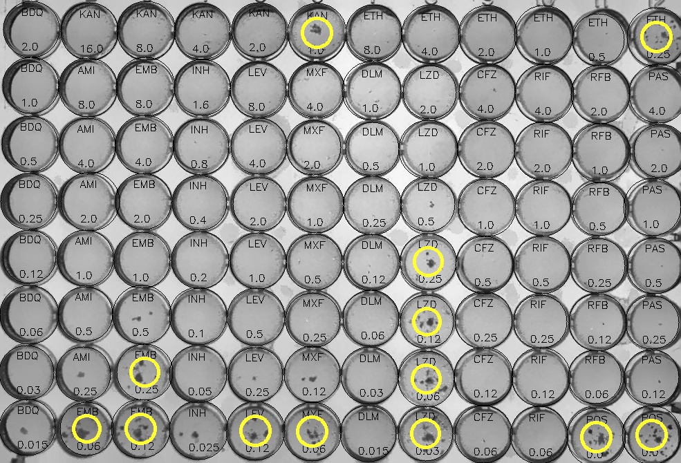 Example image of a 96-well plate that has been analysed by AMyGDA. A yellow circle means the software has classified that well as containing bacterial growth.[/caption]
Citing
Please cite
Automated detection of bacterial growth on 96-well plates for high-throughput drug susceptibility testing of Mycobacterium tuberculosis
Philip W Fowler, Ana Luiza Gibertoni Cruz, Sarah J Hoosdally, Lisa Jarrett, Emanuele Borroni, Matteo Chiacchiaretta, Priti Rathod, Sarah Lehmann, Nikolay Molodtsov, Clara Grazian, Timothy M Walker, Esther Robinson, Harald Hoffmann, Timothy EA Peto, Daniela Maria M. Cirillo, E Grace Smith, Derrick W Crook
Microbiology (2018) 164:1522-1530 doi:10.1099/mic.0.000733
Installation
This is python3; python2 will not work. Installation is straightforward using the included setup.py script. The code is freely available via GitHub on condition that you agree to the conditions in the included LICENCE.md file. First clone the repository (or download it directly from the GitHub page) $ git clone https://github.com/Philip Fowler/amygda.git This will download the repository, creating a folder on your computer called amygda/. If you only wish to install the package in your $HOME directory (or don't have sudo access) issue the --user flag. $ cd amygda/ $ python setup.py install --user Alternatively, to install system-wide $ sudo python setup.py install The setup.py will automatically looks for the required following python packages and, if they are not present, will install them, or if they are an old version, will update them. The prerequisites are described in more detail in the README.md of the AMyGDA repository on GitHub.
Tutorial
The code is structured as a python module; all files for which can be found in the amygda/ subfolder.
ls
LICENCE.md                   amygda/                       setup.py
README.md                    examples/                     bin/
config/
You may see other folders like build/ if you are run the setup.py script. To run the tutorial move into the examples/ sub-folder
$ cd examples/
$ ls
sample-images/
analyse-plate-with-amygda.py is a simple python file showing how the module can be used to analyse a single image. The fifteen images shown in Figure S1 in the Supplement of the accompanying paper (see above) are provided so you can reconstruct Figures S2, S3, S4 & S12. The images are organised as follows
$ ls sample-images/
01 02 03 04 05 06 07 08 09 10 11 12 13 14 15

$ ls sample-images/01/
image-01-raw.png
To process and analyse a single image using the default settings is simply
$ analyse-plate-with-amygda.py --image sample-images/01/image-01-raw.png And should take no more than 10 seconds. No output is written to the terminal, instead you will find a series of new files have been written in the samples-images/01 folder.
$ ls -a sample-images/01/
.datreant/
image-01-arrays.npz
image-01-mics.txt
image-01-msf.jpg
image-01-clahe.jpg
image-01-filtered.jpg
image-01-growth.jpg
image-01-raw.png- The hidden
.datreantfolder contains twoJSONfiles.categories.jsoncontains all the MICs and other metadata about the plate and both can be automatically discovered and read using thedatreantmodule to make systematic analyses simpler. image-01-mics.txtcontains the same information as theJSONfile but in a simpler format that is easier for humans to read.image-01-arrays.npzcontains a series ofnumpyarrays that specify e.g. the percentage growth in each wellimage-01-raw.pngis the original image of the plate.image-01-msf.jpgis a JPEG of the plate following mean shift filteringimage-01-clahe.jpgis a JPEG of the plate following mean shift filtering and then a Contrast Limited Adaptive Histogram Equalization filter to improve contrast and equalise the illumination across the plate.image-01-filtered.jpgis a JPEG of the plate following both the above filtering operations and a histogram stretch to ensure uniform brightness.image-01-growth.jpgadds some annotation; specifically the locations of the wells are drawn, each well is labelled with the name and concentration of drug and wells which AMyGDA has classified as containing bacterial growth are highlighted with a coloured circle.
To see the other options available for the analyse-plate-with-amygda.py python script
$ ./python analyse-plate-with-amygda.py --help
usage: analyse-plate-with-amygda.py [-h] [--image IMAGE]
                                [--growth_pixel_threshold GROWTH_PIXEL_THRESHOLD]
                                [--growth_percentage GROWTH_PERCENTAGE]
                                [--measured_region MEASURED_REGION]
                                [--sensitivity SENSITIVITY]
                                [--file_ending FILE_ENDING]

optional arguments:
  -h, --help        show this help message and exit
  --image IMAGE     the path to the image
  --growth_pixel_threshold GROWTH_PIXEL_THRESHOLD
                    the pixel threshold, below which a pixel is
                    considered to be growth (0-255, default=130)
  --growth_percentage GROWTH_PERCENTAGE
                    if the central measured region in a well has
                    more than this percentage of pixels labelled as
                    growing, then the well is classified as growth
                    (default=2).
  --measured_region MEASURED_REGION
                    the radius of the central measured circle, as a
                    decimal proportion of the whole well
                    (default=0.5).
  --sensitivity SENSITIVITY
                    if the average growth in the control wells is
                    more than (sensitivity x growth_percentage),
                    then consider growth down to this sensitivity
                    (default=4)
  --file_ending FILE_ENDING
                    the ending of the input file that is stripped.
                    Default is '-raw'
To analyse all plates, you can either use a simple bash loop
$ for i in 01 02 03 04 05 06 07 08 09 10 11 12 13 14 15; do analyse-plate-with-amygda.py --image sample-images/$i/image-$i-raw.png; done;Alternatively if you have GNU parallel installed you can use all the cores on your machine to speed up the process.
$ find sample-images/ -name '*raw.png' | parallel analyse-plate-with-amygda.py --image {} To delete all the output files, thereby returning sample-images/ to its clean state, a bash script is provided. Use with caution!
$ cd samples-images/

$ ls 01/
image-01-mics.txt                image-01-msf.jpg
image-01-arrays.npz              image-01-growth.jpg
image-01-clahe.jpg               image-01-raw.png
image-01-filtered.jpg

$ bash remove-output-images.sh

$ ls 01/
image-01-raw.png
Adapting for different plate designs
AMyGDA is written to be agnostic to the particular design of plate, or even the number of wells on each plate. The concentration (or dilution) of drug in each well is defined by a series of plaintext files in
config/For example the drugs on the UKMYC5 plate (a variant of the Thermo Fisher MYCOTB plate) is defined within the
config/CRyPTIC1-V1-drug-matrix.txtfile and looks like.
BDQ,KAN,KAN,KAN,KAN,KAN,ETH,ETH,ETH,ETH,ETH,ETH
BDQ,AMI,EMB,INH,LEV,MXF,DLM,LZD,CFZ,RIF,RFB,PAS
BDQ,AMI,EMB,INH,LEV,MXF,DLM,LZD,CFZ,RIF,RFB,PAS
BDQ,AMI,EMB,INH,LEV,MXF,DLM,LZD,CFZ,RIF,RFB,PAS
BDQ,AMI,EMB,INH,LEV,MXF,DLM,LZD,CFZ,RIF,RFB,PAS
BDQ,AMI,EMB,INH,LEV,MXF,DLM,LZD,CFZ,RIF,RFB,PAS
BDQ,AMI,EMB,INH,LEV,MXF,DLM,LZD,CFZ,RIF,RFB,PAS
BDQ,EMB,EMB,INH,LEV,MXF,DLM,LZD,CFZ,RIF,POS,POS
Adding a new plate design is simply a matter of creating new files specifying the drug, concentration and dilution of each well. Note that changing the number of wells at present also involves specifying the well_dimensions when creating a PlateMeasurement object. Currently this defaults to (8,12) i.e. a 96-well plate in landscape orientation. As an example, the configuration files for the UKMYC6 plate, which is the successor to the UKMYC5 plate, are included although all the provided examples are of UKMYC5 plates.